

Bell Curve Definition: Normal Distribution Meaning Example in Finance
A bell curve is a standard variable distribution type known as the normal distribution. The term “bell curve” originates from the graph used to depict a normal distribution consisting of a symmetrical bell-shaped curve.
The highest point on the curve, or the top of the bell, represents the most probable event in a series of data points (its mean, mode, and median). At the same time, all other possible occurrences are symmetrically distributed around the mean, creating a downward-sloping curve on each side of the peak. The standard deviation of the bell curve serves to describe its width.
Understanding a Bell Curve
The term “bell curve” describes a graphical depiction of a normal probability distribution whose underlying standard deviations from the mean create the curved bell shape. A standard deviation is a measurement used to quantify the variability of data dispersion in a set of given values around the mean. The mean, in turn, refers to the average of all data points in the data set or sequence and will be found at the highest point on the bell curve.
Financial analysts and investors often use a normal probability distribution when analyzing a security’s returns or overall market sensitivity. In finance, standard deviations that depict a security’s returns are known as volatility.
For example, stocks that display a bell curve are usually blue-chip stocks with lower volatility and more predictable behavioral patterns. Investors use the normal probability distribution of a stock’s past returns to make assumptions about future returns.
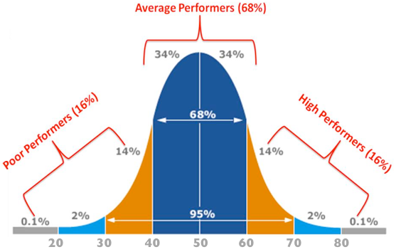
In addition to teachers who use a bell curve when comparing test scores, the bell curve is often also used in the world of statistics, where it can be widely applied. Bell curves are also sometimes employed in performance management, placing employees who perform their jobs in an average fashion in the normal distribution of the graph. The dropping slope represents the highest and lowest performers on either side. It can be helpful in larger companies when doing performance reviews or making managerial decisions.
Example of a Bell Curve
A bell curve’s width is defined by its standard deviation, which is calculated as the level of variation of data in a sample around the mean. Using the empirical rule, for example, if 100 test scores are collected and used in a normal probability distribution, 68% of those test scores should fall within one standard deviation above or below the mean. Moving two standard deviations away from the mean should include 95% of the 100 test scores collected. Moving three standard deviations away from the mean should represent 99.7% of the scores (see the figure above).
Test scores that are extreme outliers, such as 100 or 0, would be considered long-tail data points that lie squarely outside the three-standard deviation range.
Bell Curve vs. Non-Normal Distributions
However, the average probability distribution assumption doesn’t always hold in the financial world. It is feasible for stocks and other securities to sometimes display non-normal distributions that fail to resemble a bell curve.
Non-normal distributions have fatter tails than a bell curve (average probability) distribution. A fatter tail skews negative signals to investors that there is a greater probability of negative returns.
Limitations of a Bell Curve
Grading or assessing performance using a bell curve forces groups of people to be categorized as poor, average, or sound. For smaller groups, categorizing a set number of individuals in each category to fit a bell curve will do a disservice to the individuals. Sometimes, they may all be just average or even good workers or students, but given the need to fit their rating or grades to a bell curve, some individuals are forced into the poor group. In reality, data is not perfectly regular. Sometimes, there is skewness, or a lack of symmetry, between what falls above and below the mean. Other times, there are fat tails (excess kurtosis), making tail events more probable than the normal distribution would predict.
What are the characteristics of a bell curve?
A bell curve is a symmetric curve centered around the mean, or average, of all the data points being measured. The standard deviation determines the width of a bell curve; 68% of the data points are within one standard deviation of the mean, 95% of the data points are within two standard deviations, and 99.7% of the data points are within three standard deviations of the mean.
How is the bell curve used in finance?
Analysts will often use bell curves and other statistical distributions when modeling different potential outcomes that are relevant for investing. Depending on the analysis being performed, these might consist of future stock prices, rates of future earnings growth, potential default rates, or other vital phenomena. Before using the bell curve in their analysis, investors should carefully consider whether the outcomes being studied are, in fact, normally distributed. Failing to do so could seriously undermine the accuracy of the resulting model.
What Are the Limitations of the Bell Curve?
Although the bell curve is a useful statistical concept, its applications in finance can be limited because financial phenomena—such as expected stock-market returns—do not fall neatly within a normal distribution. Therefore, relying too heavily on a bell curve when predicting these events can lead to unreliable results. Although most analysts are well aware of this limitation, it is relatively complex to overcome this shortcoming because it is often unclear which statistical distribution to use as an alternative.
Conclusion
- A bell curve is a graph depicting the normal distribution, which has a shape reminiscent of a bell.
- The top of the curve shows the mean, mode, and median of the data collected.
- Its standard deviation depicts the bell curve’s relative width around the mean.
- Bell curves (normal distributions) are commonly used in statistics, including analyzing economic and financial data.

